Study of Support Vector Machines

Introduction to support vectors

In machine learning, support vector machines (SVMs, also support vector networks) are supervised learning models with associated learning algorithms that analyze data used for classification and regression analysis.

What are support vectors

Support vectors are the data points that lie closest

to the decision surface (or hyperplane)

• They are the data points most difficult to classify

• They have direct bearing on the optimum location

of the decision surface

• We can show that the optimal hyperplane stems

from the function class with the lowest

“capacity”= # of independent features/parameters

Theoretical concept

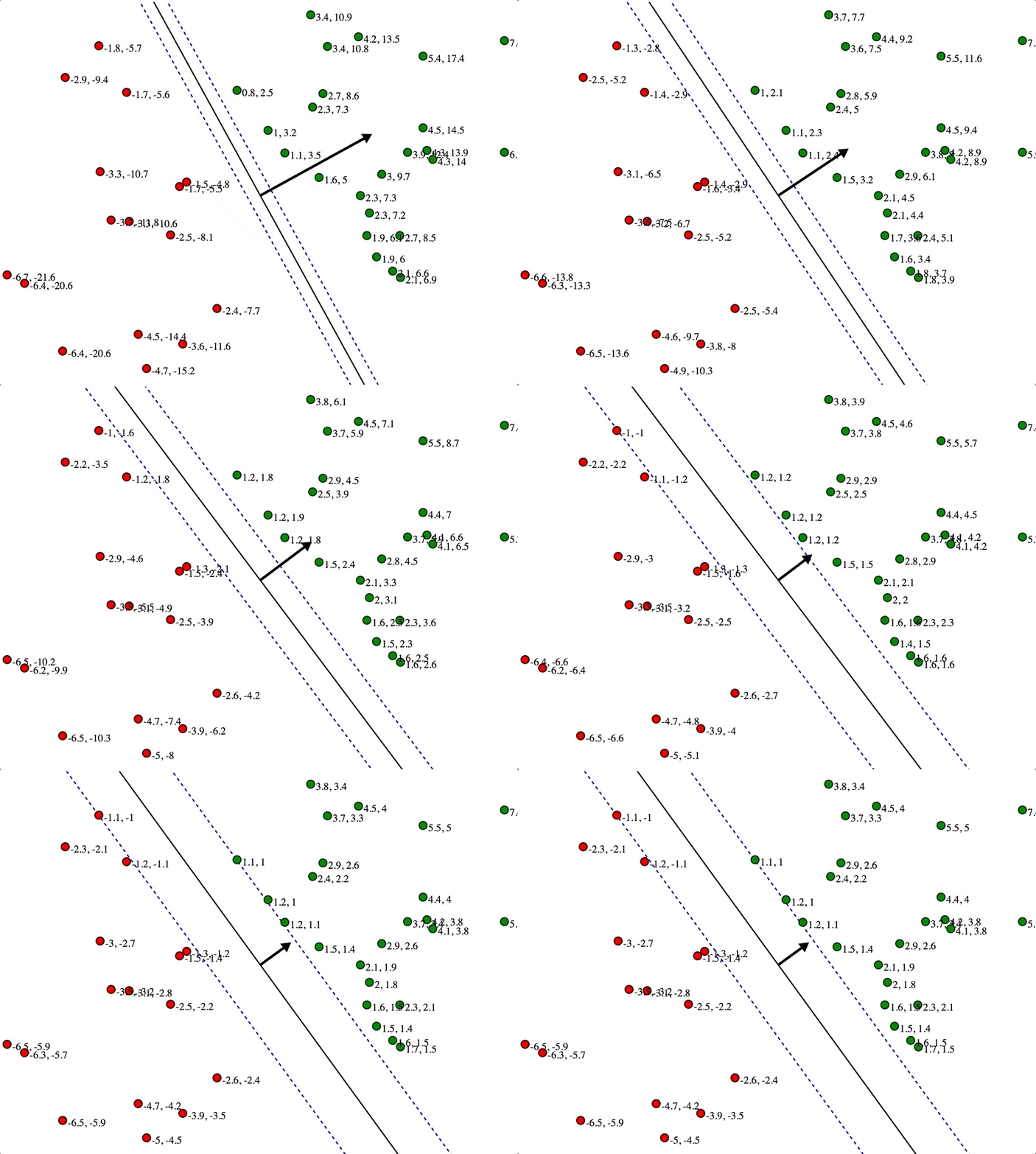
SVMs maximize the margin (Winston terminology: the ‘street’) around the separating hyperplane. 

• The decision function is fully specified by a (usually very small) subset of training samples, the support vectors. 

• This becomes a Quadratic programming problem that is easy to solve by standard methods

Separation by Hyperplanes

• Assume linear separability for now

• in 2 dimensions, can separate by a line

– in higher dimensions, need hyperplanes

In general

Input: set of (input, output) training pair samples; call the input sample features x1, x2…xn, and the output result y. Typically, there can be lots of input features xi 

Output: set of weights w (or wi ), one for each feature, 

whose linear combination predicts the value of Y

Important difference: we use the optimization of maximizing the margin (‘street width’) to reduce the number of weights that are nonzero to just a few that correspond to the important features that ‘matter’ in deciding the separating line(hyperplane)

These nonzero weights correspond to the support vectors (because they ‘support’ the separating hyperplane)

Defining the separating Hyperplane

• Form of equation defining the decision surface separating

the classes is a hyperplane of the form:wTx + b = 0

– w is a weight vector

– x is input vector

– b is bias

• Allows us to write

wTx + b ≥ 0 for di = +1

wTx + b < 0 for di = –1

Maximizing the margin (aka street width)

We want a classifier (linear separator)

 with as big a margin as possible.

Recall the distance from a point(x0,y0) to a line:

Ax+By+c = 0 is: |Ax0 +By0 +c|/sqrt(A2+B2), so,

The distance between H0 and H1 is then:

|w•x+b|/||w||=1/||w||, so

The total distance between H1 and H2 is thus: 2/||w||

In order to maximize the margin, we thus need to minimize ||w||. With the

condition that there are no datapoints between H1 and H2:xi

•w+b ≥ +1 when yi  =+1  xi 

•w+b ≤ –1 when yi  =–1 

Both Can be combined into: yi (xi •w) ≥ 1

Criteria

Suppose there exists a hyperplane w >x + b = 0 such that

- w T x n + b ≥ 1 for yn = +1 

- w T x n + b ≤ −1 for yn = −1 

- Equivalently, yn(w T x n + b) ≥ 1 ∀n (the margin condition)

- Also note that min1≤n≤N |w T x n + b| = 1 

- Thus margin on each side: γ = min1≤n≤N  |w T xn+b| / ||w|| = 1 /||w|| 

- Total margin = 2γ = 2 /||w||

Alpha in svm

Lagrangian multiplier, usually denoted by α is a vector of the weights of all the training points as support vectors.

Suppose there are m training examples. Then α is a vector of size m. Now focus on any ith element of α: αi. It is clear that αi captures the weight of the ith training example as a support vector. Higher value of αi means that ith training example holds more importance as a support vector

Method of Lagrange multipliers states that J is minimized for w and b as before, but it has to be maximized for α. The point that J represents is called a saddle point.

Variations in data

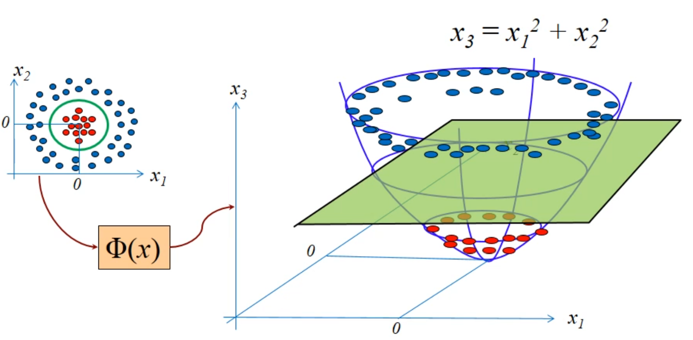
SVMs can also learn nonlinear decision boundaries using kernels. In the SVM classifier, it is easy to have a linear hyper-plane between these two classes. But, another burning question which arises is, should we need to add this feature manually to have a hyper-plane. No, the SVM algorithm has a technique called the kernel trick. 

The SVM kernel is a function that takes low dimensional input space and transforms it to a higher dimensional space i.e. it converts not separable problem to separable problem. It is mostly useful in non-linear separation problem. Simply put, it does some extremely complex data transformations, then finds out the process to separate the data based on the labels or outputs you’ve defined

1. Noisy data

For noisy data, we introduce a training error parameter in our estimation/optimization. We introduce a slack variable and add the extra condition as

2. Non linear Boundry

Any data set which has a non-linear boundary would be theoretically linearly separable if projected to higher dimensions.

Now if we look the data closely in 3D we can find that we can create a partition based on a given condition Hence Q(α) can we written as:

Svm in Python

Here we will use the sklearn support vector to use an example

 We have three models to use that are SVC, NuSVC and LinearSVC. In this implementation we will use SVC

Code

# X of shape (n_samples, n_features)

# Y is the target 

from sklearn import svm

X = [[0, 0], [1, 1]]

y = [0, 1]

clf = svm.SVC()

clf.fit(X, y)

#Output 

#SVC()

# Now we predict the value from clf model

clf.predict([[2., 2.]])

#Output

#array([1])

# get support vectors

clf.support_vectors_

#Output

#array([[0., 0.],

       [1., 1.]])

# get indices of support vectors

clf.support_

#Output

#array([0, 1]...)

# get number of support vectors for each class

clf.n_support_

#Output

#array([1, 1]...)

More information on each of SVM model is given in the link